Key Considerations: Part 1
Preparative Chromatography Course
1 - Fundamentals of Preparative Chromatography
3 - Preparative Chromatography Instrumentation
4 - Key Considerations: Part 1
5 - Key Considerations: Part 2
6 - Column Selection
7 - Automated Preparative Purification Instrumentation - UFPLC
8 - Automatic Analytical to Preparative Scale Up
9 - Triggering Fractionation
10 - Preparative SFC
11 - Course Summary & Test

Key Considerations: Part 1
Welcome to Course Unit 4: Key Considerations of Preparative Chromatography.
This section will cover how to scale your analysis, understanding the objectives of the separation, critical parameters for loading studies and operation parameter considerations. Hopefully by the end of this section, you should understand some of the important points which needs to be addressed to successfully perform preparative chromatography.
Separation Objectives and Resolution
For most analysts, the aim for prep analysis is purifying a target compound cheaply and quickly.
It is important to establish the required quantity as well as the purity of that yield. For example, a chemist might require 700 mg of synthesised product at a purity of greater than 95%. This has implications for devising the methodology and what stationary phase format is required. If the loading capacity isn’t sufficient for the stationary phase used, it will take longer to achieve the 700 mg, whilst if the chromatography hasn’t provided adequate resolution between the peak of interest and impurities, then the purity can be compromised. Let’s look at this in more detail.
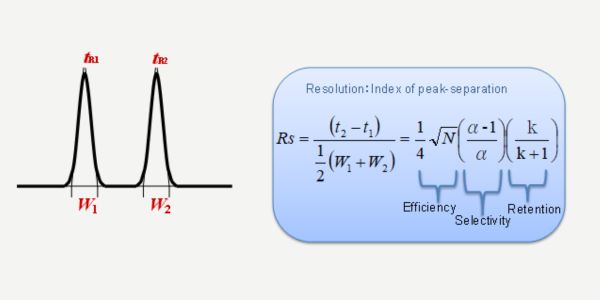
The main peak of interest must be resolved sufficiently to avoid contaminating that fraction with any undesired impurities. Resolution is calculated as shown in Figure 1, where it considers the retention time and peak width of the pair. Resolution is a combination of efficiency, selectivity and retention, where the largest impact on resolution is selectivity. Column efficiency is not as important in preparative chromatography as in analytical chromatography. Provided the peak of interest is resolved from the other peaks, we are not usually concerned about the chromatography for the other compounds which might be in the mixture.
Peak Overloading and Scale-UP Considerations
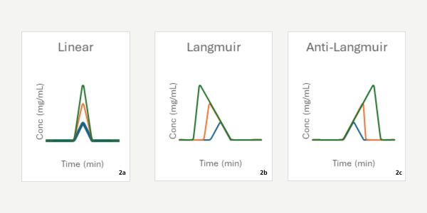
The aim for analytical chromatograms is to obtain sharp, Gaussian peaks, however, within preparative chromatography, peaks are overloaded and therefore often asymmetrical. As the concentration or load increases, each analyte has a different response. Some have a linear increase as concentration rises (2a), however, the most prevalent case is the Langmuir isotherm (2b). The Langmuir adsorption isotherm leads to significant peak tailing with an increase in concentration and an earlier shift in the peak apex, where more compound is found in the mobile phase than in the stationary phase. This is due to the analyte exceeding the stationary phase’s capacity. For completeness, another common loading phenomenon is the Anti-Langmuir isotherm (2c), where there is considerable peak fronting, and the compound resides for longer in the stationary phase with increasing concentration. It is important to understand the overloading profile of your compound, as this helps explain where in the chromatogram you ideally want the peak of interest to elute, so that impurities do not appear underneath it as the load increases. It also helps explain why greater resolution than is typically achieved on the analytical scale is needed when moving from low load to the broader, overloaded peak associated with preparative scale.
Loading Studies
As previously highlighted, the amount of sample analysed is critical. The more sample that can be loaded onto the column means fewer injections are required to acquire the same yield. However, stationary phases have a maximum loading capacity beyond which efficiency declines. If the column capacity is exceeded, it can cause a phenomenon where a portion of the analyte migrates through the column without interacting with the stationary phase. This can result in unfavourable peak shapes, such as broadening and spitting, which can have negative implications for preparative separations. Loading studies are used to investigate this and are performed in one of two ways: concentration load or injection load.
Since there are concerns about reproducibility near the load limit, it is advisable to allow for some margin within these studies.
|
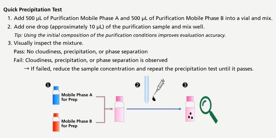
Figure 3. Quick Precipitation Test for Assessing Sample Solubility Prior to Preparative Chromatography |
The injection amount should be kept constant, whilst the concentration varies from low to high in a step-by-step approach. Whilst the impact of the sample solvent is diminished during a concentration load study, there is the potential for precipitation along the flow path with increasing concentration. A quick precipitation test will help understand the influence of mobile phase on the compound of interest. Figure 3 provides a three-step process to determine whether there is any precipitation or phase separation in the mobile phase.
|
| Pros | Cons |
|---|---|
| The impact of the sample solvent is smaller compared to the injection load. | Depending on the solubility, precipitation may occur within the flow path. |
|
|
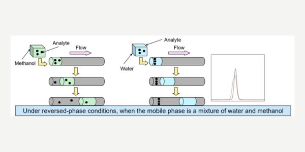
This is investigated by varying the injection amount in stages using the same concentration sample. When increasing the injection volume, it is necessary to pay special attention to the effect of the sample solvent. It is necessary to pay special attention to the effect of the sample solvent. In cases where the sample solvent has a stronger elution power than the mobile phase, the peak shape may deteriorate depending on the injection volume (a tendency to exhibit leading – the red trace in the chromatogram in Figure 4). For example, in reversed phase mode, a high proportion of methanol can often lead to detrimental peak shape. When the sample diluent is weaker than the elution strength of the mobile phase, the peak is not adversely affected by broadening. Since it greatly depends on the column internal diameter, it is important to pay attention to the injection volume when reducing the column ID.
|
| Pros | Cons |
|---|---|
| The risk of precipitation for the sample is low. |
The analysis time varies based on the suction amount It is susceptible to the effects of the sample solvent. There are limitations on the system used (such as specifications for maximum injection volume). |

Maximising Sample Loading
Let’s look at an example of why we would want to maximise on loading.
We’ve been given an isocratic analytical method, which contains two compounds, A and B (figure 5). The aim of the separation is to isolate and collect 700 mg of peak A at a purity of greater than 92%, but not compound B. The analytical method employs a 250 x 4.6 mm,5 μm C18 column with an injection volume of 5 μL.
We have high solubility of the sample in our injection solvent and after making a concentrated solution, we can recover approximately 1 mg of compound A for a 30 minute run time with a purity of greater than 99%. Although the purity is very high, the yield and the rate is too low, therefore we need to increase the load. If we were to carry out our LC purification on this analytical scale column, at this loading we would be looking at 34 injections and 17 hours.
Increasing Injection Volume
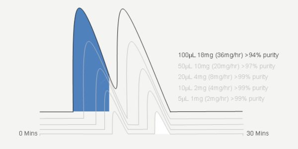
If we increase the injection volume on our analytical column, from 5 to 10 μL, we double the yield, with ample purity (Figure 6.). Another increase to 20 μL means we now can achieve 8 mg/hour with >99% purity. When we reach 50 μL, the rate achievable is 20 mg/hour, with >97% purity, which is meeting our requirements. At an injection volume of 100 μL, the peaks are no longer baseline resolved, which is compromising the purity but still acceptable. As such, we can no longer increase the injection volume and expect to achieve acceptable purity, and we can still only obtain 36 mg/hour. This means it would take 39 injections and 19 hours to achieve the desired yield and purity. The analytical scale has gone as far as is practical.
Scaling Up the Method
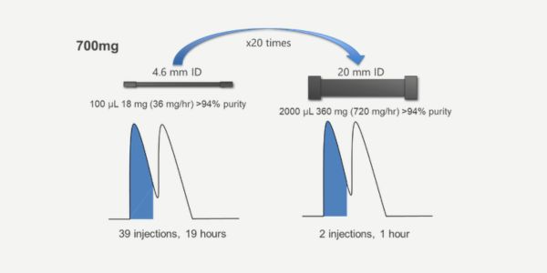
To improve the rate of this purification, we should scale up to a larger ID, column, but one of the same length, phase and particle size. We have an instrument which can flow up to 20 mL/min, and we can translate to a 20 mm ID column with the same stationary phase, column length and particle size as the analytical method column. Scaling from a 4.6 mm ID column to a 20 mm ID column is approximately a 20 times increase in cross sectional area. Therefore, a 20x increase in injection volume, flow rate and amount of material on column should provide the same resolution of peaks. Now with a 2 mL injection volume on the 20 mm ID column, we can purify our 700 mg of compound A in greater than 94% purity in 2 injections or 1 hour.
That concludes the first of this two-part course unit on key considerations. Next time we will continue to look at other key aspects to the success of a preparative analysis including the effect of different mobile phases, understanding your analyte properties for making decisions and solutions to common issues.
Your Shimadzu Chromatography Team
Related Resources
-
-
Watch short videos explaining analytical intelligence features of Shimadzu HPLC systems
-