Column Selection
Preparative Chromatography Course
1 - Fundamentals of Preparative Chromatography
3 - Preparative Chromatography Instrumentation
4 - Key Considerations: Part 1
5 - Key Considerations: Part 2
7 - Automated Preparative Purification Instrumentation - UFPLC
8 - Automatic Analytical to Preparative Scale Up
9 - Triggering Fractionation
10 - Preparative SFC
11 - Course Summary & Test

Column Selection
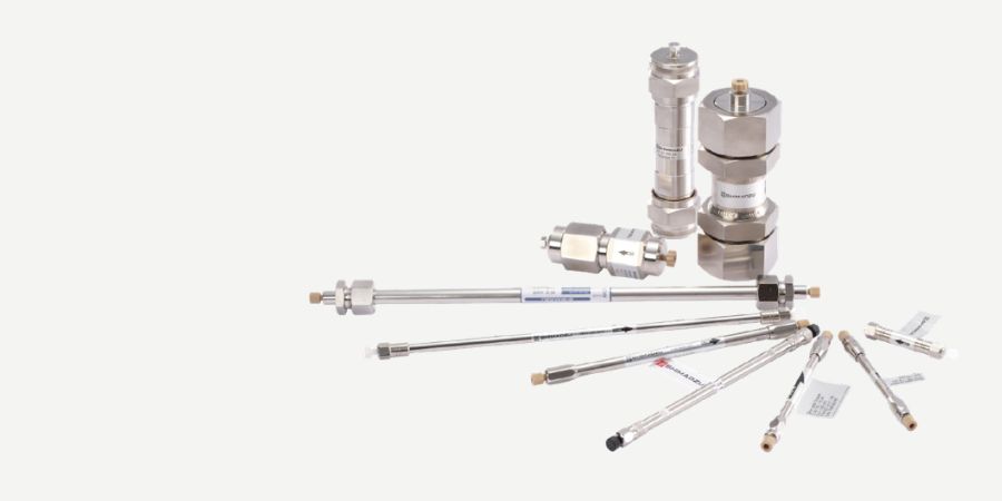
Figure 1. Key Parameters Influencing Preparative HPLC Method Development
Welcome back for this section on selecting stationary phases for preparative analysis. Previously we looked at some of the most common questions and considerations related to prep HPLC.
Separation Mode Selection

First it is important to establish which separation mode is required for the type of sample which needs to be analysed. The most common mode is reversed phase, however, it is sometimes necessary to use alternative modes such as normal phase, size exclusion or ion exchange, which all have different primary retention mechanisms. For example, reversed phase chromatography employs polar solvents and non-polar stationary phases for a predominant hydrophobic retention mechanism.
The stationary phase should be selected based on the structure of the target compound (size, charge, functional groups), physicochemical properties (logP/D, pKa), and types of impurity components (analogues, synthetic raw materials, decomposable products etc).
Stationary phase parameters to consider include:
| Property | Rationale |
|---|---|
| Ligand functionality |
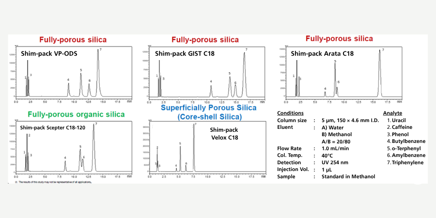
It is important to know that the same “type” of column might have significantly different selectivity profiles. As displayed in Figure 1, the chromatographic profile of five C18 columns are vastly different and wide retention windows. It is also worthwhile trying different ligand functionalities to provide alternative selectivity profiles.
Variability in Selectivity Across Different C18 HPLC Columns |
| Pore size | With the increase in biomolecular applications, it is important to select the right pore size. Large molecules need larger pore sizes to accommodate their hydrodynamic volume, so they have sufficient accessibility to interact with the stationary phase. Compounds with a molecular weight less than 4000 Daltons usually can be analysed on a 60-120 Å, whereas, above that weight, a 300 Å. The surface area is inversely proportionate to the pore diameter larger surface area also changes the amount of loading capacity. |
| Scalability between analytical and prep column formats | If the ligand isn’t available in the prep format, then the desired yield will take substantially longer to achieve. |
| Particle size | Efficiency isn’t as critical for preparative separations, as the sample is substantially overloaded. With analytical separations, most applications aim for smaller, more efficient particle sizes, however, preparative applications typically employ 5-10 μm. |
| Loading capacity | We discussed loading capacities in the previous section in more detail. However, it is important to remember that if we exceed the loading capacity of the column then we could experience breakthrough which can cause adverse effects for our chromatography, recovery and purity. |
| Internal diameter | HPLC applications usually employ 4.6 mm column internal diameters; however, this is usually increased to ~10 mm ID for semi-prep and ~21 mm ID for preparative scale, which allows for much greater velocities through the column thus increasing the throughput. |
Scaling Injection Volume and Flow Rate
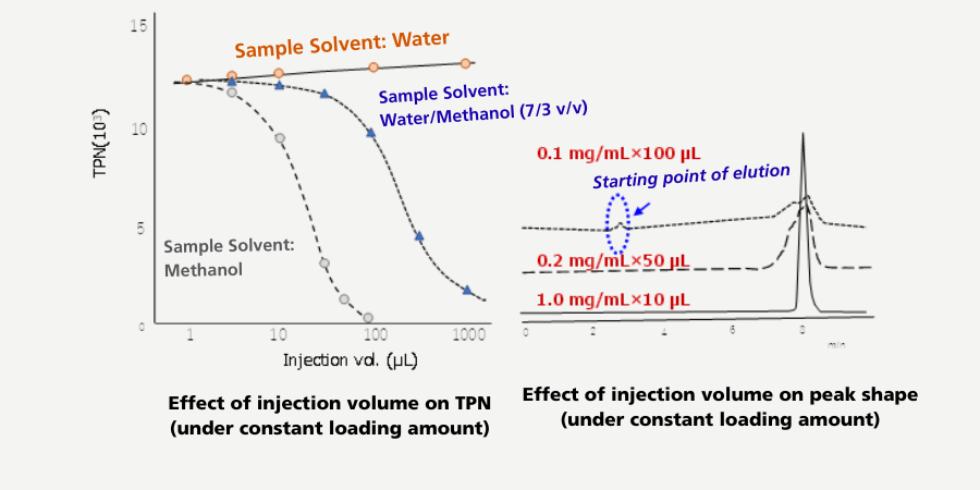
Scaling up can impact on the run time, solvent consumption and suitable yield in a reasonable timeframe. However, the scale up may be limited by the sample solubility and injection volume. This can result in poor chromatographic performance and poor peak shapes, which can impact on the success of the fraction collection. It is also important to optimise the sample diluent to prevent a loss of performance or deterioration of peak shape, which could be attributed to poor sample interaction with the stationary phase.
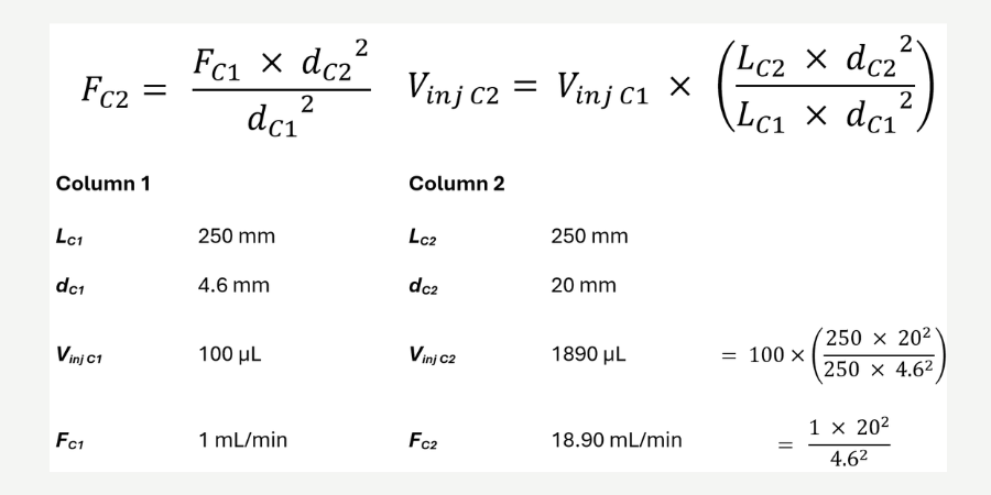
Take this figure. The analytical scale can achieve a load of 18 mg using a 100 μL injection volume. To achieve 650 mg of sample, it would take approximately 18 ½ hours. By utilising preparatory conditions, the load can be increased to approximately 340 mg using an 1890 μL injection volume, thus reducing the analysis time to just 1 hour. This is a significant saving in time and resources.
Scaling Factors for Preparative Chromatography
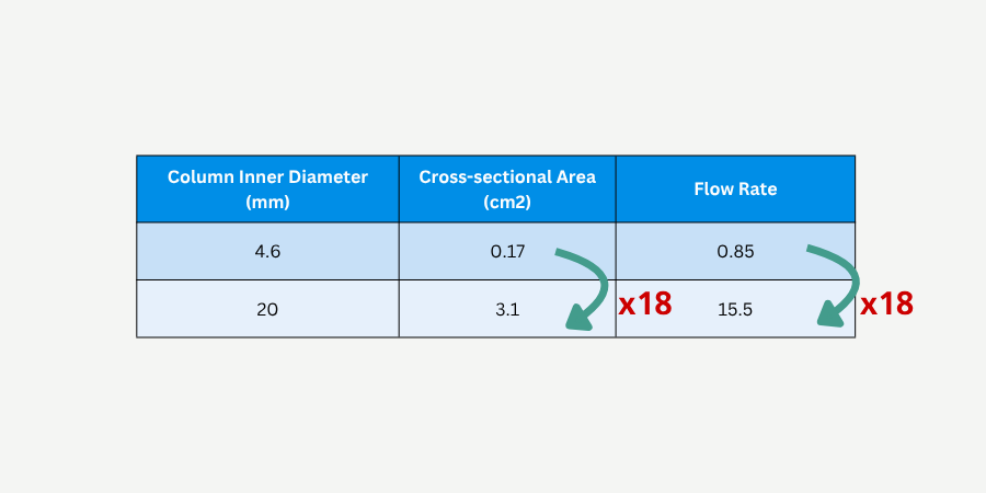
The simplest translation would consist of keeping the particle size the same between the column used on the analytical scale and the prep scale. This means only the flow rate needs to change to suit the column’s internal diameter when using the same particle size.
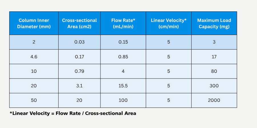
The below table gives examples of scale-up based on the sizes of the columns used during method development and the dimensions for the fractionation column. If the same particle size columns are used during both method development and fractionation, flow rate calculations become easier.
Method Transfer for Preparative LC

The example beside illustrates an isocratic separation on the analytical and preparative scale. The top chromatogram has a 5 mg/mL sample delivered in a 100 μL injection, on a ShimPack Scepter C18, 250 x 4.6 mm, 5 μm particles. The flow rate was increased from 1 mL/min to 19 mL/min when the column was changed to a 250 x 20 mm, 5 μm columns. The injection volume was proportionately increased to 1900 μL. This increases the load on the column from 0.5 mg to 9.5 mg.
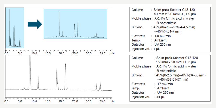
Changing the column dimensions, particle size and using gradient chromatography can add extra complications when it comes to translating the methodology to prep conditions. Figure 8 illustrates the analytical gradient separation and conditions which are then translated to the larger scale. In this example, the column format for the analytical is 50 x 3.0 mm with 1.9 μm. The prep column is a 150 x 20 mm, 5 μm formats. As such, the gradient times, flow rate and injection volume all need to be adjusted.
ShimPack Scepter Series
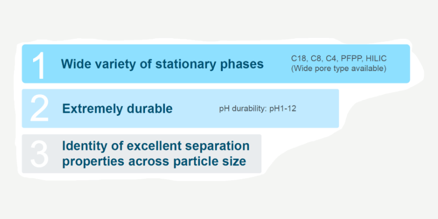
The ShimPack Scepter series is a fully scalable range of stationary phases with different ligand functionality capable of analysis over a wide pH range.
Hopefully you now have a firm understanding of the different stationary phase considerations for you to feel confident in selecting columns for preparative separations. Next time, we will be looking at a unique technology which automates the fractionation, concentration, purification and elution of compounds using UFPLC.
Best regards,
Your Shimadzu Chromatography Team
Related Resources
-
-
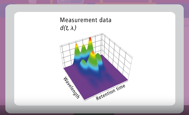
Watch short videos explaining analytical intelligence features of Shimadzu HPLC systems
-